Organ Axis model

1. Definition of distance function (D), spatial location (P), and structure (S)

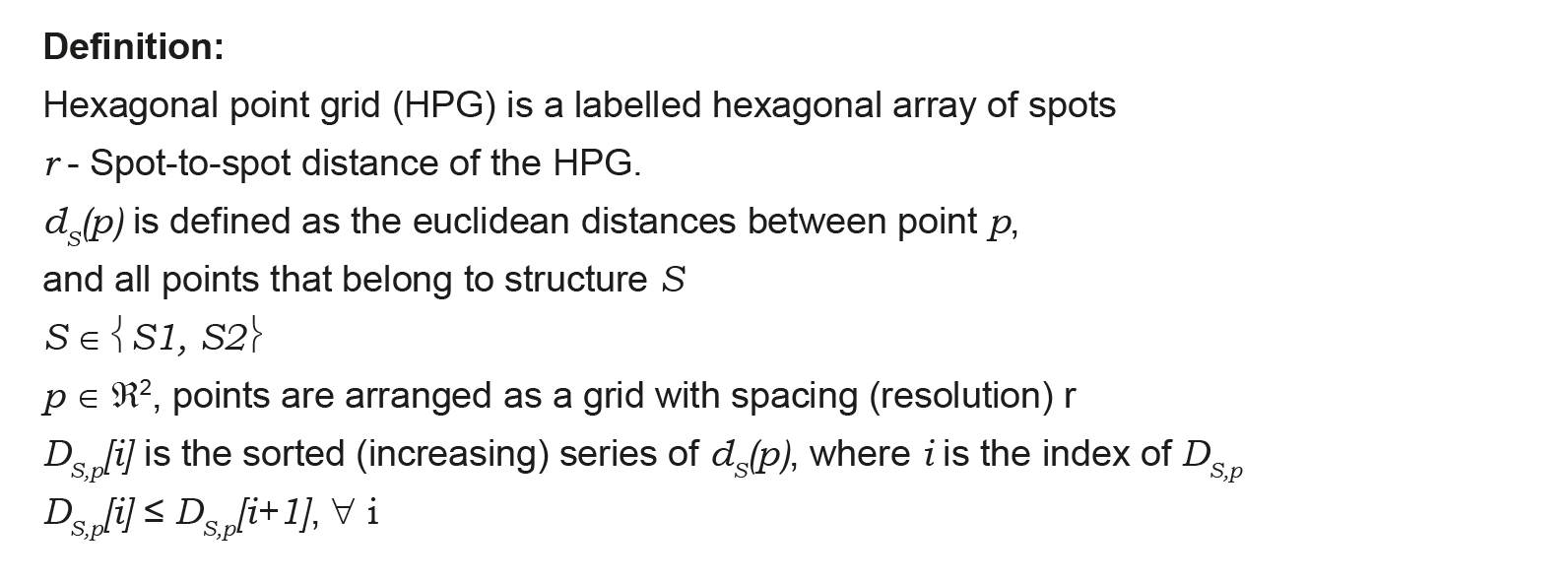
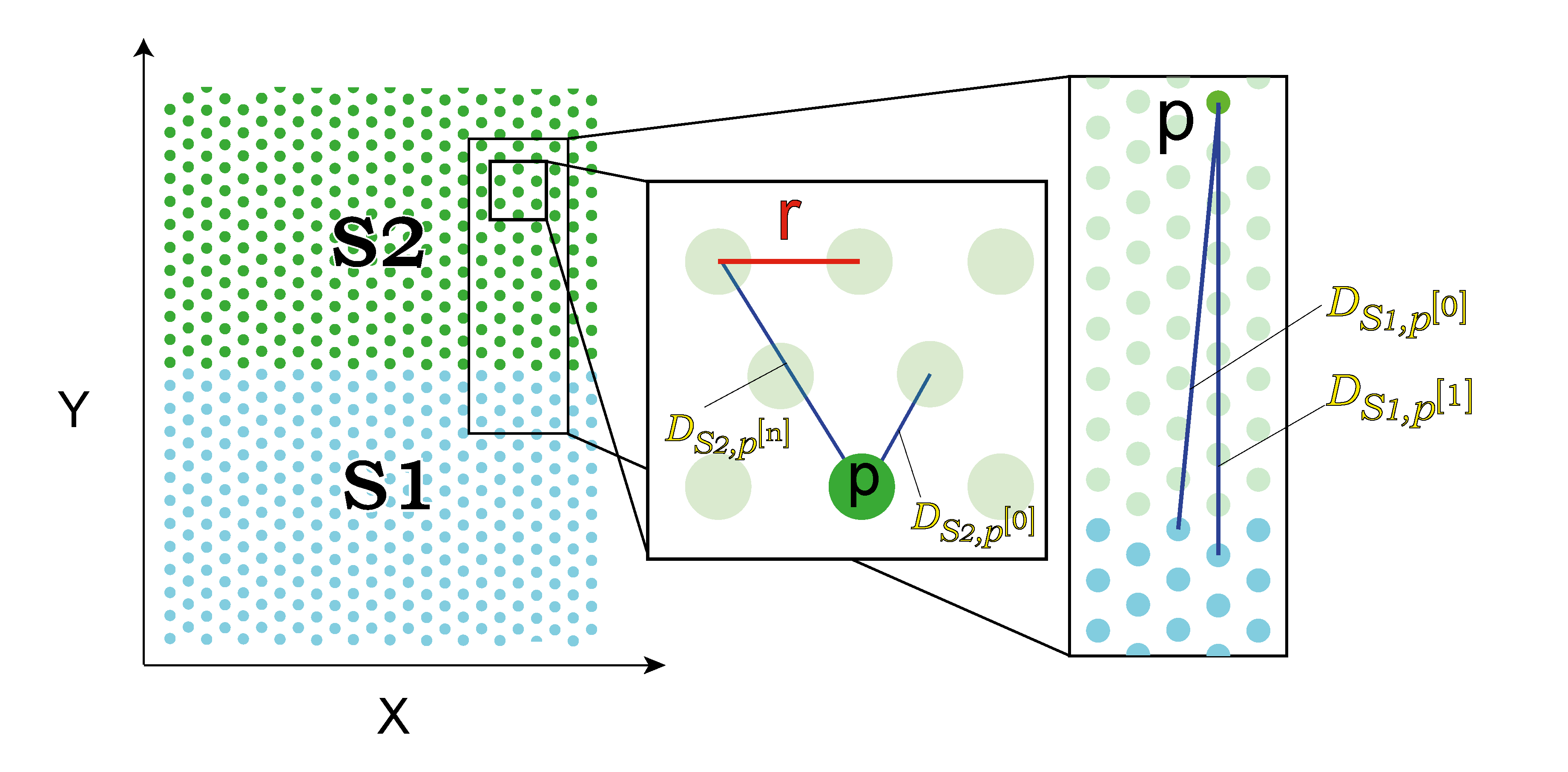
We define P as any point in space, S as a tissue region. We further establish the sampling frequency of the grid points (r) and the number of points to be considered (K). Based on these, we can define a minimal euclidean distance function (D), which calculates the minimal distances from every point P to its K nearest points in a structure S. Here we use a where P is a member of the hexagonal grid but this does not necessarily have to be the case as illustrated in the simulations below. With D defined, the mean distance from point P to structure S across a set of K nearest points is calculated. To achieve this, we introduce μ, the mean of minimal Euclidean distances to K nearest points. Subsequently, the relative signed position of any point P with respect to two structures can be computed. This is done through function H, which calculates the normalised difference between μS1 and μS2 (Supplementary Figure 2c, Equation 2). Simulations of H within respect to a linear axis parallel to S1 and S2 of H produces an S-shaped in space, bounded between -1 and 1, with 0 marking the equidistance between structures S1 and S2. The established model has two key features: Near the boundary (on in equidistance) between two regions S1 and S2 (around x = 0) the function H is most sensitive to changes in the value of P (changes in euclidean position). In this region, even a small change in P can lead to a relatively large change in output score. This sensitivity is due to the steep slope of the curve at its midpoint. For P that is further away from the boundary, towards either positive or negative infinity, the output of H gradually approaches its maximum (1) or minimum (-1) value, respectively. In these regions, the curve flattens out, hence changes in P have diminishing effects on the output score.

2. Mean distance of nearest points of S to P

With D defined, we proceed to calculate the mean distance from point P to structure S across a set of K nearest points. To achieve this, we introduce μ, the mean of minimal distances, where K represents the count of nearest points. For that we can define:

3. Inferring the normalised position relative to two structures

Subsequently, we can compute the relative (directional) position of any point P with respect to the distance to two structures. This is done through the normalised difference between μS1 and μS2. Function H describes a sigmoid in space, scaling between -1 and 1, with 0 marking the equidistance between structures S1 and S2.

Exploration and intuition from simulations of K and grid resolution on axis function

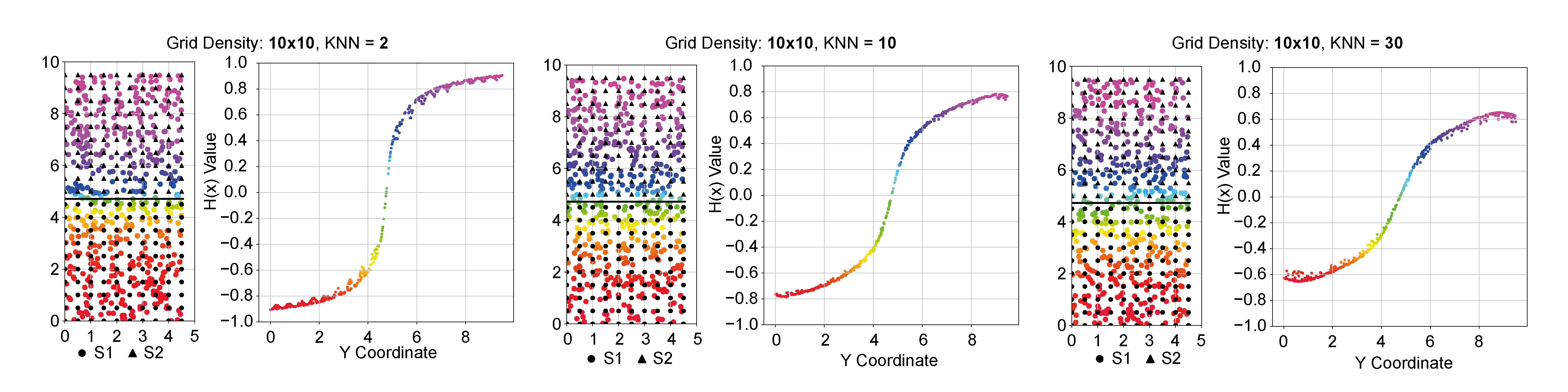
To investigate how the number of nearest points (K) or the grid density (r) influences the transformation of space into axis positions, we conducted simulations using a grid with randomly placed points within that grid. Our analysis primarily focuses on the relationship between the linear position along the Y-axis and the axis function H, distinguishing between two structures.

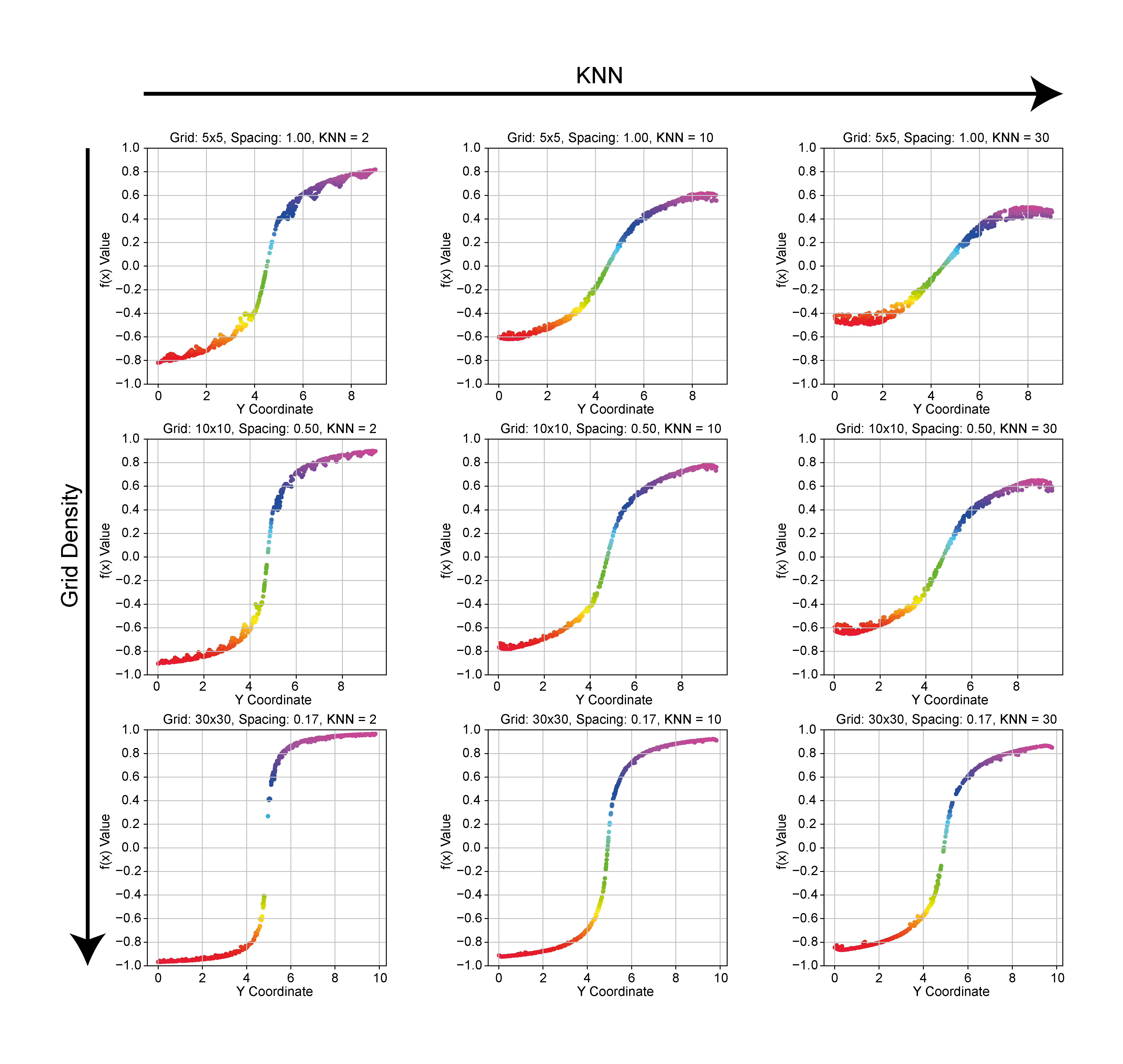
Changing the K nearest points and keeping the grid constant: With a KNN of 2, H exhibits a “jagged” appearance, likely due to the predominance of values reflecting the simulated grid square pattern. In addition H exhibits a more step-like function shape. Both of these effects are due to the increased influence of the local environment over the global position. In high K=30, H is “flattened” and the values are more continuous but we can start seeing edge effects where the score is diminished by lack of sufficient grid points at the edges, effectively increasing the average distance to the nearest K points.

Changing the grid spacing and keeping K constant: At low grid density relative to K, the dependency of H is more gradual and edge effects are visible. In the highest grid density H behaves as a full sigmoid and transitions if faster around the border.

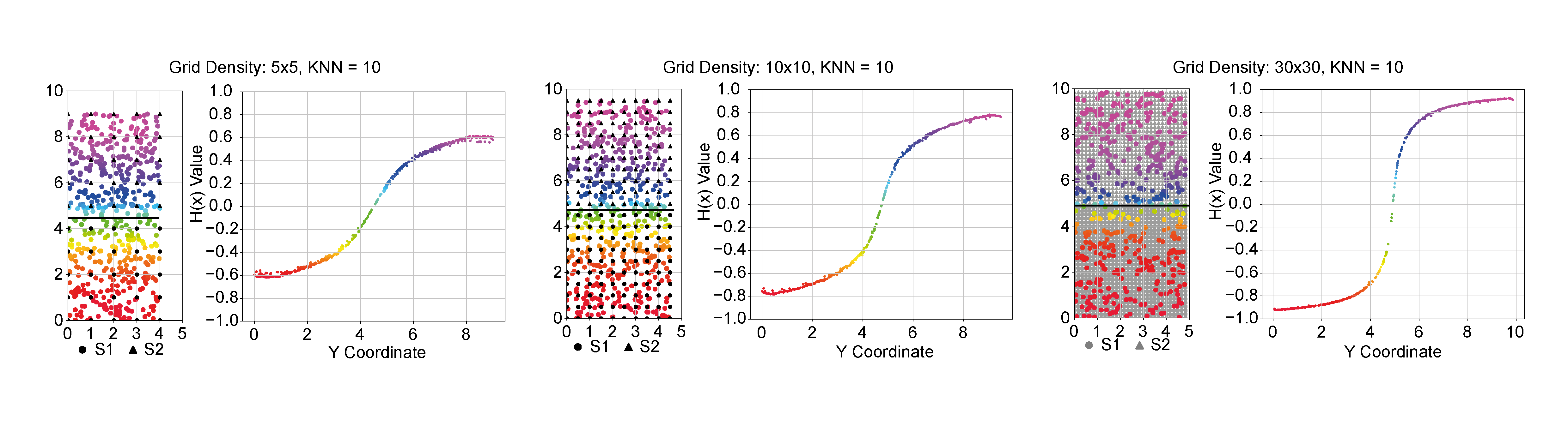
Changing both grid spacing and K in a matrix